SPACE Lab: Pulsed Plasma Thruster Stand

Summary:

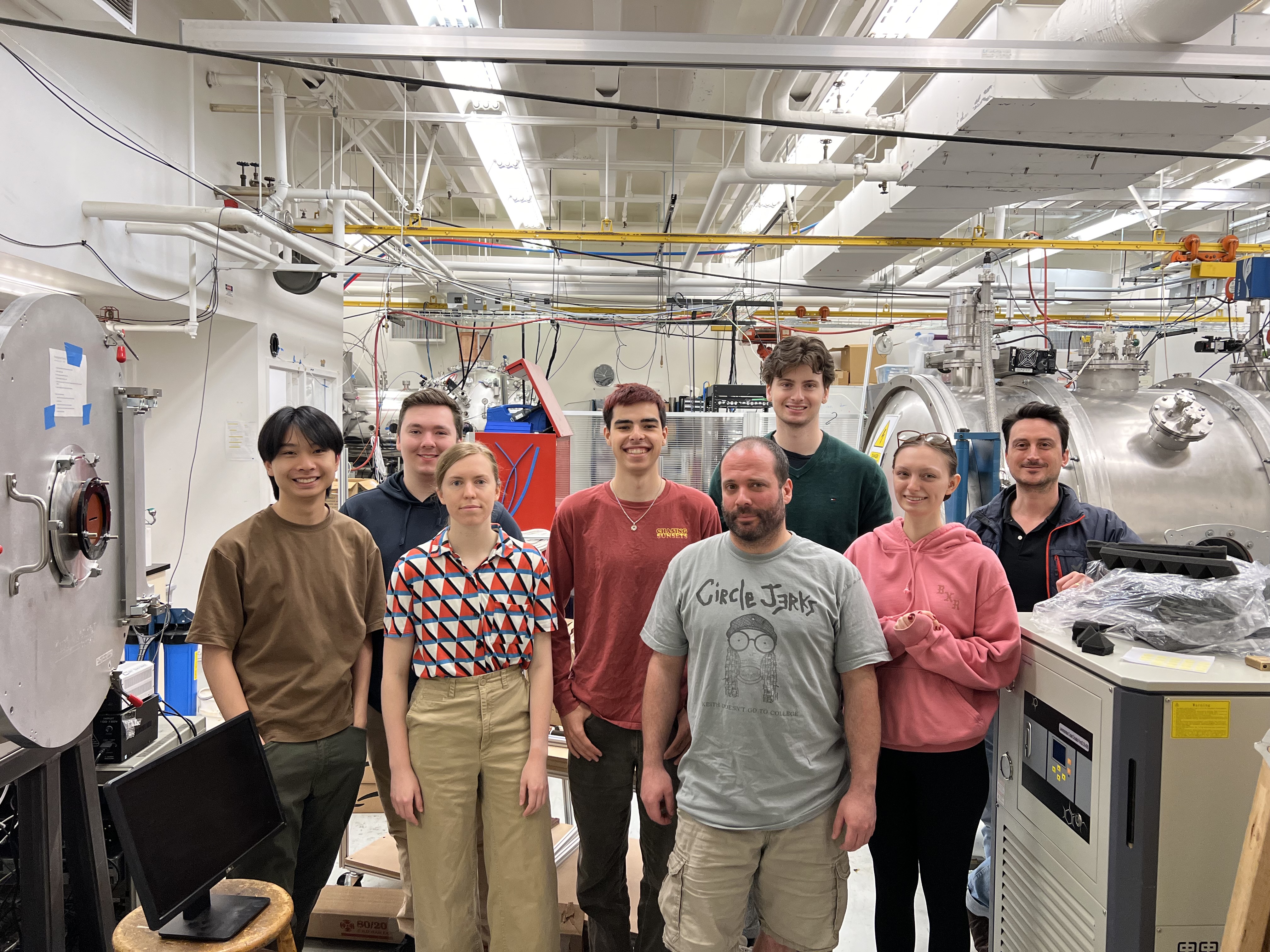
• SPACE Lab Mentor: Dr. Justin Little
• Space Lab Team: Nathan Cheng, Felicity Cundiff, Adam Delbow, Ben Fetters, Lillie LaPlace, Kai Laslett-Vigil, and Winston Wilhere
• Capstone awards showcase top work at the University of Washington, Seattle - (SPACE Lab) Here
• Space Propulsion and Advanced Concepts Engineering Laboratory at the University of Washington, Seattle - (SPACE Lab) Here

The project aimed to develop an inverted pendulum test stand for UW's SPACE Lab, intended to measure impulses from pulsed plasma thrusters ranging from 10 μNs to 100 mNs. Constructed with materials like Garolite and Delrin for stability and minimal interference, the test stand underwent rigorous reviews (PDR, CDR, TRR) to ensure it met design specifications. However, during testing, it did not achieve consistent resolution of impulses within the targeted range. This outcome highlighted challenges in accurately measuring thrust forces, necessitating further refinement and calibration to enhance its performance for future experiments in pulsed plasma propulsion research.

Mission Objective:

To design and build an operational, minimally conductive, inverted pendulum test stand for the University of Washington’s SPACE Lab. The stand should accurately resolve impulses from pulsed plasma thrusters within a range of 10 μN*s to 100 mN*s.

• 1. Preliminary Design Review (PDR): Here
• 2. Critical Design Review (CDR): Here
• 3. Test Readyness Review (TRR): Here
• 4. System Test Procedure: Here
• 5. System Test Plan: Here
• 6. Design Document: Here
• 7. Aceptance Review (AR): Here
• 8. Test Stand Technical Drawings: Here
• UW Aero Astro Youtube feature: Here
• UW Aero Astro Instagram feature: Here

Space Lab Team: Nathan Cheng, Felicity Cundiff, Adam Delbow, Ben Fetters, Lillie LaPlace, Kai Laslett-Vigil, Winston Wilhere - Mentor: Dr. Justin Little

Designed and built Inverted pendulum test stand for the University for Washington’s SPACE Lab

Preliminary Design Review (PDR)

The Preliminary Design Review (PDR) for the Pulsed Plasma Thruster Test Stand project defined the technical specifications and design requirements essential for its success. This phase focused on key aspects:

• Impulse Measurement Range: Designed to measure impulses from 10 μN*s to 100 mN*s, crucial for evaluating thruster efficiency.
• Steady-State Thrust Measurement: Capable of measuring thrusts from 0.1 mN to 0.1 N to assess thruster capabilities.
• Thruster Support Capacity: Supports thrusters up to 8 kg for flexibility in experimental setups.
• Precision in Alignment: Ensures alignment accuracy of ±0.05 degrees for reliable performance measurement.
• Zero-Point Return Accuracy: Returns to zero point with ±0.001 degrees accuracy to minimize measurement errors.

Materials like Garolite and Delrin were chosen for low outgassing, high strength, and dimensional stability, reducing EMI and ensuring measurement reliability. An inverted pendulum design enhances sensitivity to detect small forces effectively.

• Real-Time Data Processing: Software processes sensor data in real-time for immediate feedback and adjustments.
• User Interface: Intuitive interface allows easy parameter adjustment, real-time data monitoring, and efficient test environment control.
• Data Logging and Analysis: Comprehensive logging facilitates detailed analysis and supports research reproducibility.

This integration supports effective operation under various experimental conditions, advancing research in pulsed plasma propulsion.

Critical Design Review (CDR)

The Critical Design Review (CDR) for the Pulsed Plasma Thruster Test Stand project focused on finalizing the design specifications and validating the chosen approaches for system construction. This phase ensures that all components are ready for manufacturing and integration:

• Chamber Specifications:
  • Dimensions: 1.5m width x 1.5m depth x 2.0m height.
  • Volume: 4.5 cubic meters.
  • Pressure range: 0 to 1 atmosphere, controlled via digital vacuum pump capable of achieving 10^-6 Torr.
  • Temperature range: -20°C to +60°C, monitored by PT100 sensors with accuracy ±0.1°C.
  • Material: 304 stainless steel, thickness 5mm, to withstand high vacuum conditions and thermal stress.

Inverted Pendulum Type Test Stand
• Pendulum Design:
  • Length adjustable from 0.5m to 2.0m, using precision linear actuators.
  • Mass of pendulum bob: 1.0 kg, made from aluminum to reduce weight while maintaining structural integrity.
  • Sensor resolution: Encoder with 0.01-degree resolution for precise angular measurement.
  • Calibration: Using a standard mass and g-level apparatus to ensure accuracy.

Inverted Pendulum Type Test Stand

Assembly Overview
• Leveling System:
  • - Base of the test stand will be leveled by way of a stepper motor.
  • - Base will be allowed to pivot through a TBD angle on nylon bushings.
  

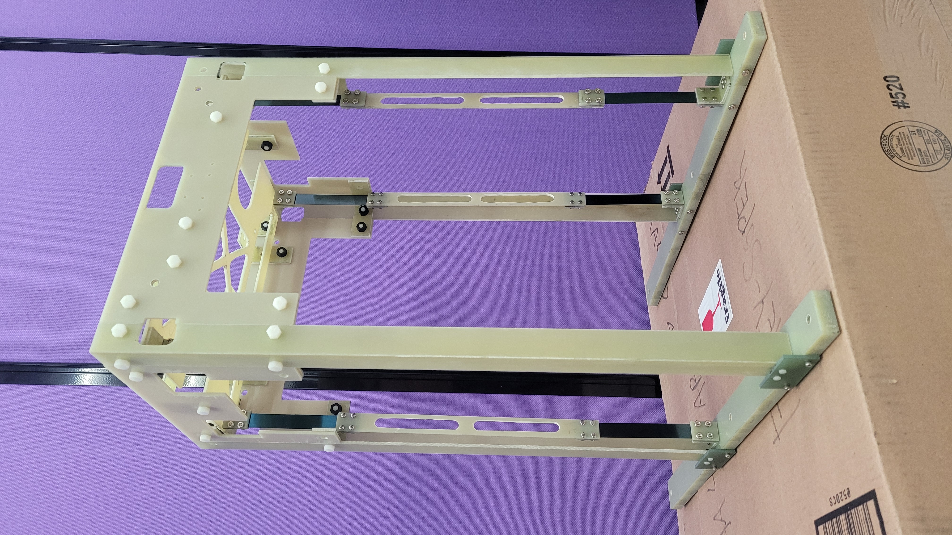
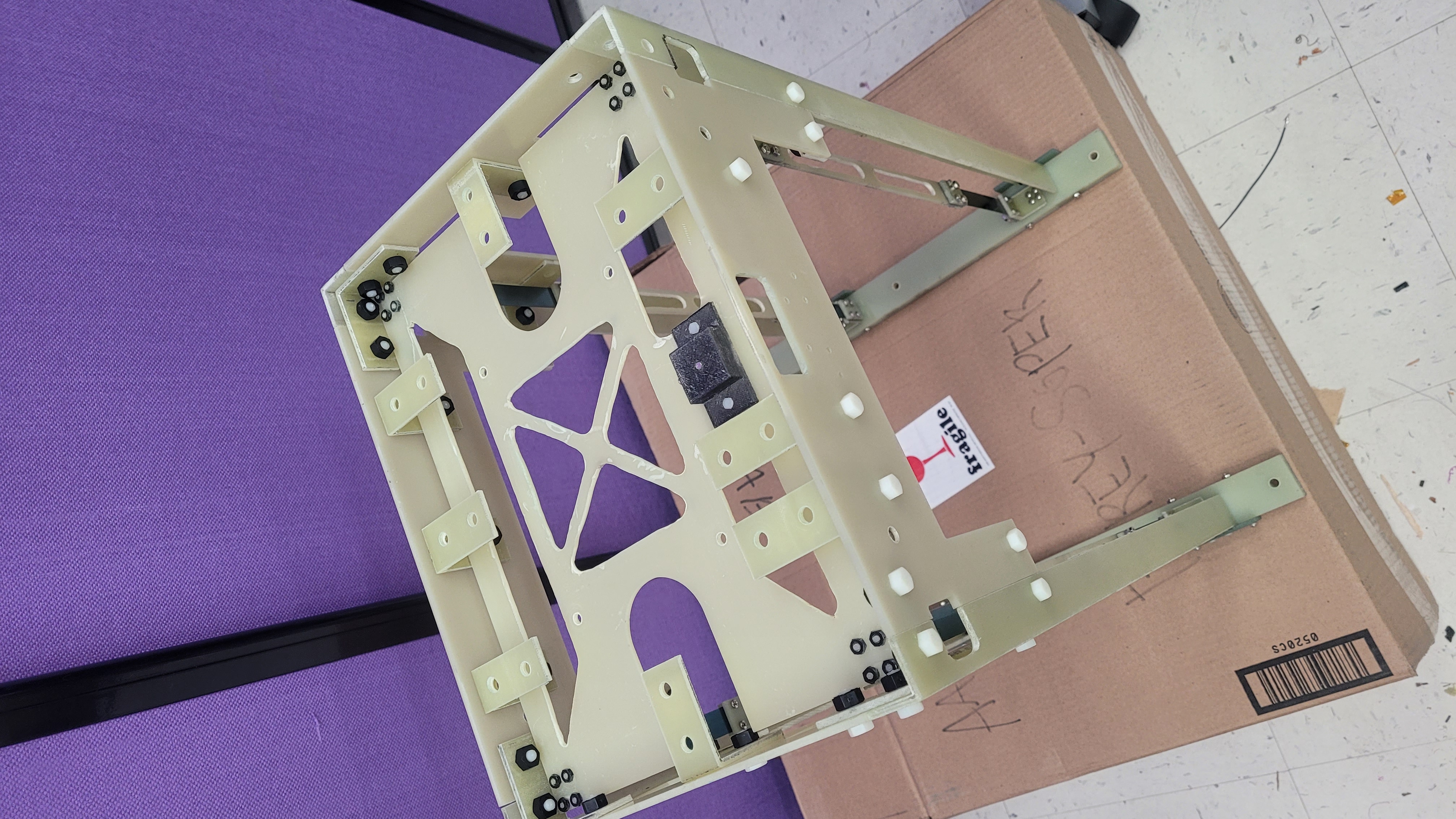
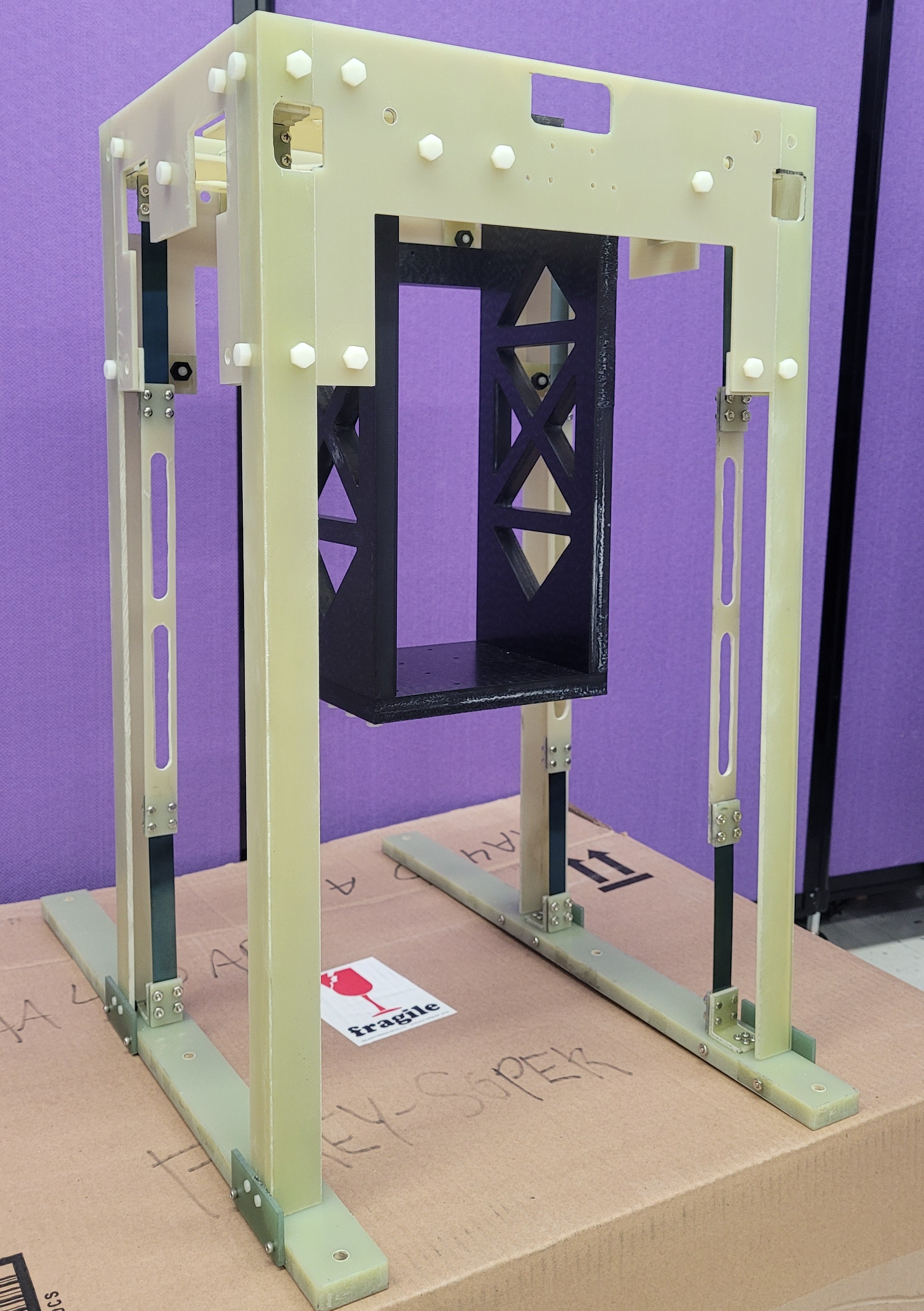
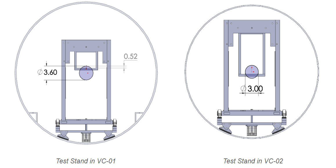
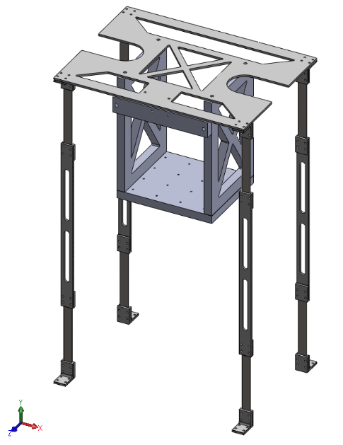
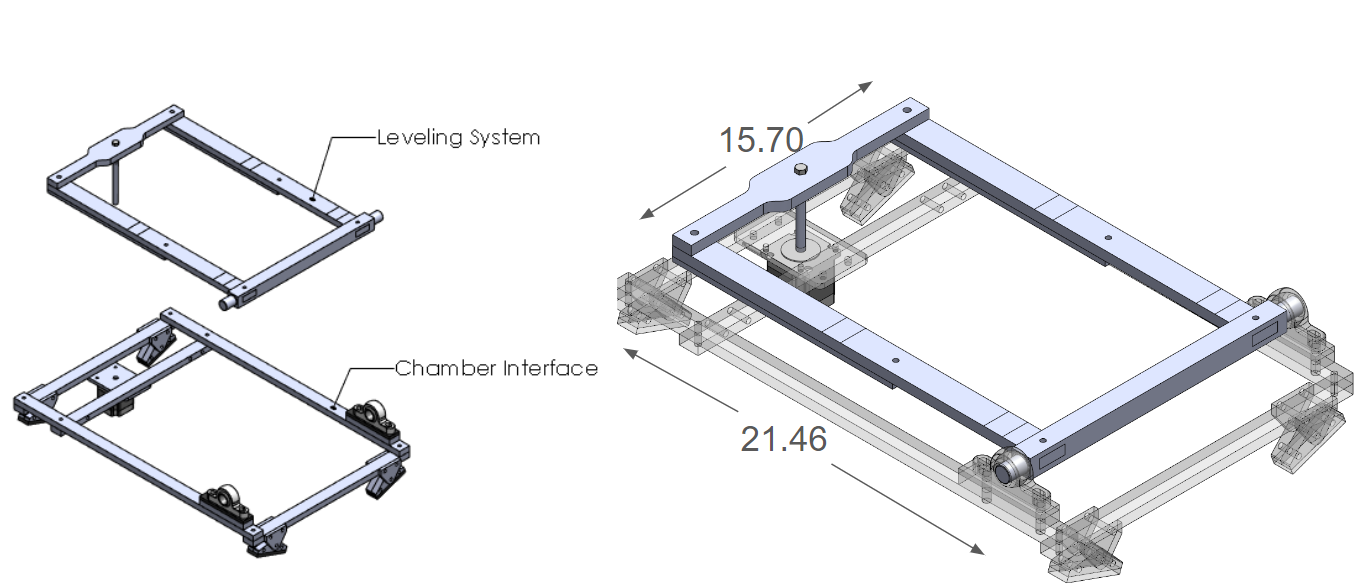  Leveling System: Structure Overview

  

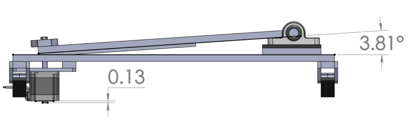  Leveling System: Able to pitch ±3 degrees
  

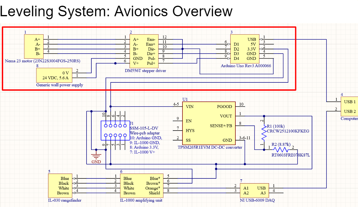  Leveling System: Avionics Overview

  

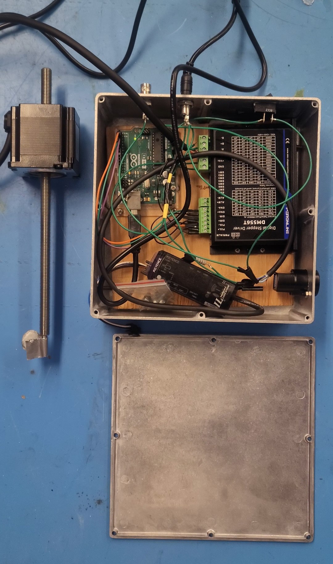
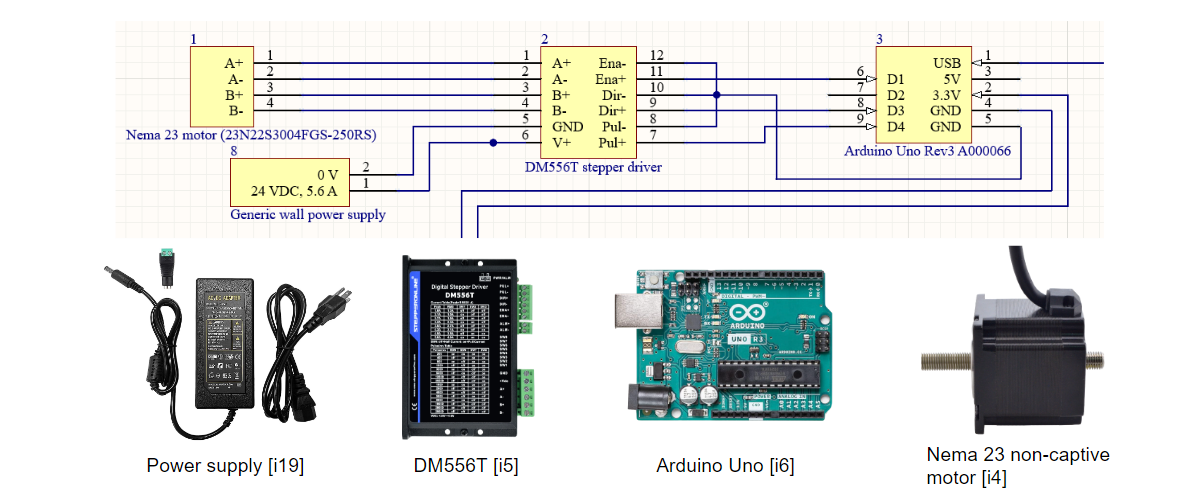  Non-captive actuator model chosen for smaller footprint compared to other design options. Nema 23 metal actuator rod converted to 3D printed part. DM556T chosen for high compatibility with Arduino Uno and Nema 23 motors.
• Thrust Measurements:
  • - Measurement range: 10 μN*s to 100 mN*s, critical for capturing the full range of thrust outputs from the PPT.
  • - Instrumentation: Use of strain gauges and laser displacement sensors for precise measurement.
  • - Calibration: Calibration against the Dawstar PPT, with accuracy expected within ±5% of actual thrust measurements.
  • - Predicted results: Accurate measurement within the specified range to validate the system's capability to measure impulse forces effectively.
  

  Thrust Measurement Avionics

  

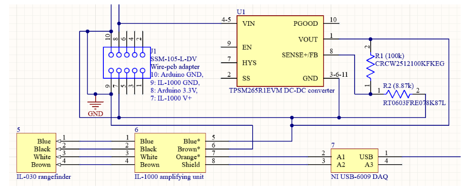
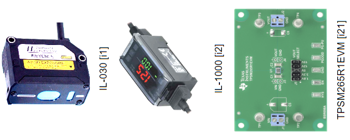  NI USB-6009 has 512 byte FIFO buffer for data transferred to the computer. IL-030 has a rated resolution of 788 μin (20 μm, to be verified) and programmable 1 - 3 kHz output frequency. IL-1000 compatible with IL-030 for signal amplification prior to digitization. TPSM265R1EVM receives 3.3V power source from Arduino and boosts it to 15V with 100mA to power IL-1000
  

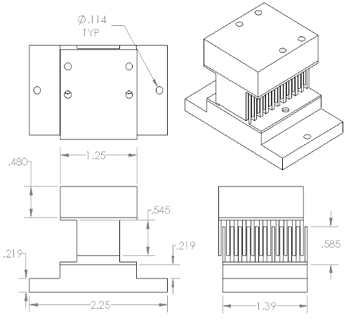  Electrostatic Comb

  

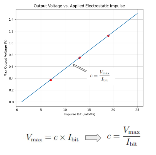  A plot of Linear Impulse is generated to determine the slope c, which represents the calibration constant of the system for the duration of testing for that day. This determination of the slope c ensures that the system's response is accurately calibrated for the specific testing conditions. The calibration process should be repeated before and after testing to ensure consistency and accuracy in the system's performance across different operating conditions.

  Calibration and Testing Code:

                              
  
      import pandas as pd
      import matplotlib.pyplot as plt
      import seaborn as sns
      from sklearn.linear_model import LinearRegression
  
      sns.set(style="whitegrid")
  
      def detect_max_voltage(csv_files, voltage_column, start_row):
          max_voltages = []  # List to store maximum voltages
          
          for csv_file in csv_files:
              print("Processing file:", csv_file)
              df = pd.read_csv(csv_file)  # Load CSV file into a DataFrame
              voltage_data = df.loc[start_row:, voltage_column]  # Select the 'CH4' column starting from row 17
              voltage_data = pd.to_numeric(voltage_data, errors='coerce')  # Convert voltage data to numeric type
              voltage_data.dropna(inplace=True)  # Drop rows with NaN values in the voltage data
              max_voltage = voltage_data.max()  # Find maximum voltage value
              max_voltages.append(max_voltage)  # Append maximum voltage to the list
              print("Maximum voltage:", max_voltage)  # Print maximum voltage value
              print()
  
          return max_voltages
  
      def plot_vmax_vs_impulses(known_impulses, max_voltages, subplot_index):
          plt.subplot(2, 1, subplot_index)  # Use the provided subplot index
          plt.plot(known_impulses, max_voltages, marker='o', linestyle='-', color='#ff5733', linewidth=3, markersize=10)  # Adjust line and marker styles
          plt.xlabel('Number of Known Impulse Plot', fontsize=14, fontweight='bold', color='#333333')  # Adjust font size and style
          plt.ylabel('Maximum Voltage', fontsize=14, fontweight='bold', color='#333333')  # Adjust font size and style
          plt.title('Linear Impulses', fontsize=16, fontweight='bold', color='#333333')  # Adjust font size and style
          plt.grid(True, linestyle='--', alpha=0.7, color='#aaaaaa')  # Adjust grid style
          plt.xticks(fontsize=12, color='#555555')  # Adjust tick labels
          plt.yticks(fontsize=12, color='#555555')  # Adjust tick labels
          plt.tight_layout()  # Adjust layout
          plt.gca().set_facecolor('#f0f0f0')  # Set background color of plot face
  
      # I_bit = v_max / c ------------------------------------------------------------------------------------------------------------------------------
      def plot_ibit_vs_vmax(max_voltages, slope, subplot_index):
          plt.subplot(2, 1, subplot_index)  # Use the provided subplot index
          bit_impulses = [v / slope for v in max_voltages]
          plt.plot(bit_impulses, max_voltages, marker='s', linestyle='--', color='blue', linewidth=2, markersize=8)  # Adjust line and marker styles
          plt.xlabel('Time (s)', fontsize=14, fontweight='bold', color='#333333')  # Adjust font size and style
          plt.ylabel('Maximum Voltage', fontsize=14, fontweight='bold', color='#333333')  # Adjust font size and style
          plt.title('Impulse Plot', fontsize=16, fontweight='bold', color='#333333')  # Adjust font size and style
          plt.grid(True, linestyle='--', alpha=0.7, color='#aaaaaa')  # Adjust grid style
          plt.xticks(fontsize=12, color='#555555')  # Adjust tick labels
          plt.yticks(fontsize=12, color='#555555')  # Adjust tick labels
          plt.tight_layout()  # Adjust layout
          plt.gca().set_facecolor('#f0f0f0')  # Set background color of plot face
  
      # File
      csv_files = ['C:/Users/every/OneDrive/Desktop/CODE/4 - PPT/CALI/T0298.csv', 'C:/Users/every/OneDrive/Desktop/CODE/4 - PPT/CALI/T0299.csv', 'C:/Users/every/OneDrive/Desktop/CODE/4 - PPT/CALI/T0299_2.csv']
      new_csv_files = ['C:/Users/every/OneDrive/Desktop/CODE/4 - PPT/CALI/T0298_I_bit.csv', 'C:/Users/every/OneDrive/Desktop/CODE/4 - PPT/CALI/T0299_I_bit.csv', 'C:/Users/every/OneDrive/Desktop/CODE/4 - PPT/CALI/T0299_2.csv']
  
      voltage_column = "CH4"  # Adjust column name as needed
      start_row = 17  # Adjust the starting row as needed
  
      known_impulses = [1, 2, 3, 4]  # Extend known impulses to 3 and 4
  
      # Detect maximum voltages for the initial CSV files
      max_voltages = detect_max_voltage(csv_files, voltage_column, start_row)
  
      # Calculate the slope using linear regression
      model = LinearRegression()
      X = pd.DataFrame(known_impulses[:len(max_voltages)])  # Ensure known impulses match the length of max_voltages
      y = pd.DataFrame(max_voltages)
      model.fit(X, y)
      slope = model.coef_[0][0]
  
      # Print the slope
      print("Slope value:", slope)
  
      # Plot both graphs on the same figure
      plt.figure(figsize=(10, 12))  # Adjust figure size
  
      # Plot V_max vs Known Impulses in the first subplot
      plot_vmax_vs_impulses(known_impulses[:len(max_voltages)], max_voltages, 1)
  
      # Detect maximum voltages for the new CSV files (if different from initial)
      new_max_voltages = detect_max_voltage(new_csv_files, voltage_column, start_row)
  
      # Plot I_bit vs V_max in the second subplot
      plot_ibit_vs_vmax(new_max_voltages, slope, 2)
  
      plt.show()    
                              
                              

  • Software GUI Features:
    • Sampling Rate: 1000 samples/second
    • Data Storage: Logs data for 24 hours (86,400,000 data points)
    • Real-time Data Processing: Provides immediate feedback
    • User-friendly GUI: Developed with Python and Tkinter
    • Control Features:
      • Controls Arduino-driven stepper motor using PySerial
      • Manages data with NI-DAQmx Driver and PySerial
      • Converts measurements to thrust values
      • Estimates thrust uncertainties
      • Calibrates deflection to thrust
      • Includes directional buttons, RPM sliders, and angle indicators
  • Materials: Garolite and Delrin chosen for low outgassing, high strength, stability, and low friction properties to minimize interference and ensure accurate measurements. Inverted pendulum design enhances sensitivity for detecting small forces effectively.
  • Integration with Test Stand: Integrates chamber, pendulum, and software for cohesive experiments under varied conditions
  • Data Logging and Analysis: Logs data for 24 hours, supporting detailed analysis
  • User Interface: GUI facilitates parameter setting, real-time data monitoring, and environment control

  This setup ensures effective operation of the Pulsed Plasma Thruster Test Stand for experimental research in pulsed plasma propulsion.

  

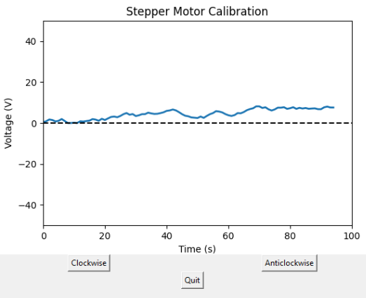  Stepper motor control GUI

  

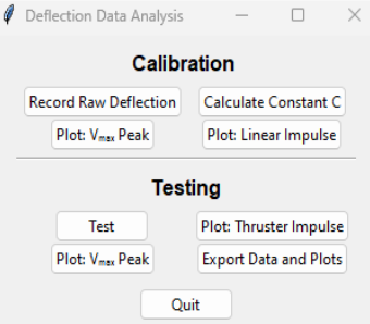  Data Analysis GUI Command Window

  Leveling Systems Python Code:

                          
      import serial
      import serial.tools.list_ports
      import tkinter as tk
      import math
      
      def move_custom(direction, degrees):
          global current_steps, step_counter_label, current_degrees  # Declare variables as global
          steps_per_revolution = 200 #confirm this empirically
          mm_per_revolution = 1.37 #confirm this empirically
          lever_arm = 20 #inches
          inch_to_mm = 25.4
          degress_to_rad = math.pi/180
          
          steps=math.sin(degrees*degress_to_rad)*lever_arm/(mm_per_revolution/inch_to_mm)*steps_per_revolution
          
          if direction == 'Up':  # Check if the direction is forward
              current_steps += steps  # Increment the current position by the number of steps
              current_degrees +=degrees
              command = 'A' + str(steps) + '\n'  # Command for forward movement
          elif direction == 'Down':
              current_steps -= steps  # Decrement the current position by the number of steps
              current_degrees -=degrees
              command = 'B' + str(steps) + '\n'  # Command for backward movement
          #print(f"Sending command: {command}")  # Debug print
          ser.write(command.encode())  # Send the command to Arduino
          step_counter_label.config(text=f"Angular position: {current_degrees}")  # Update the step counter
      
      # Function to stop everything immediately
      def stop_all():
          ser.write(b'S\n')  # Send the stop command to Arduino
          ser.flush()  # Flush the serial buffer to ensure the command is sent immediately
      
      # Function to move motor to zero position
      def move_to_zero():
          global current_steps, current_degrees  # variable global
          if current_steps >=0:  # Check if there are steps needed to move to zero
              command= 'B' + str(abs(current_steps)) + '\n'  # Command to move backward to zero position
              ser.write(command.encode())
          elif current_steps <0:
              command= 'A' + str(abs(current_steps)) + '\n' # Command to move backward to zero position
              ser.write(command.encode())
          current_steps = 0  # Reset current position
          current_degrees = 0
          step_counter_label.config(text="Angular position: 0")  
      
      # Function to quit
      def quit_app():
          move_to_zero() 
          ser.close()  
          root.quit()  
      
      # GUI setup
      def create_gui():
          global root, current_steps, step_counter_label, current_degrees  # Declare root as a global variable
          root = tk.Tk()
          root.title("Stepper Motor Control")
          current_steps = 0
          current_degrees=0
      
          custom_button = tk.Button(root, text="Move (degrees)", command=custom_steps)
          custom_button.grid(row=0, columnspan=2, padx=10, pady=10)
      
          quit_button = tk.Button(root, text="Quit", command=quit_app)
          quit_button.grid(row=1, columnspan=2, padx=10, pady=10)
      
          step_counter_label = tk.Label(root, text="Angular position: 0")
          step_counter_label.grid(row=2, columnspan=2, padx=10, pady=10)
      
          root.mainloop()
      
      # Function for custom steps input
      def custom_steps():
          custom_window = tk.Toplevel(root)
          custom_window.title("Move (degrees)")
      
          direction_label = tk.Label(custom_window, text="Direction:")
          direction_label.grid(row=0, column=0, padx=10, pady=10)
      
          direction_var = tk.StringVar(value="Up")
          direction_menu = tk.OptionMenu(custom_window, direction_var, "Up", "Down")
          direction_menu.grid(row=0, column=1, padx=10, pady=10)
      
          steps_label = tk.Label(custom_window, text="Degrees:")
          steps_label.grid(row=1, column=0, padx=10, pady=10)
      
          steps_entry = tk.Entry(custom_window)
          steps_entry.grid(row=1, column=1, padx=10, pady=10)
      
          confirm_button = tk.Button(custom_window, text="Move", command=lambda: move_custom(direction_var.get(), int(steps_entry.get())))
          confirm_button.grid(row=2, columnspan=2, padx=10, pady=10)
      
      # Arduino port
      def get_arduino_port():
          ports = serial.tools.list_ports.comports()
          for port in ports:
              if 'COM3' in port.device: 
                  return port.device
          return None
      
      # Main
      arduino_port = get_arduino_port()
      if arduino_port:
          ser = serial.Serial(arduino_port, baudrate=9600, timeout=1)
          create_gui()
      else:
          print('Arduino not found on any port!')
                              
                          

  Leveling Systems Arduino Code:

                          
      const int stepPin = 2; // Step pin connected to Arduino digital pin 2
      const int dirPin = 3;  // Direction pin connected to Arduino digital pin 3
      const int enPin = 4; // Enable pin
      
      void setup() {
      stepper.setMaxSpeed(3000); // Set maximum speed
      Serial.begin(9600); // Initialize serial communication
      digitalWrite(dirPin, HIGH);
      //digitalWrite(4, HIGH); //LOW is on?
      }
      
      void loop() {
      if (Serial.available() >= 2) { // Check if there are enough bytes available
          String str = Serial.readString(); // Read the command sent from Python
          String command = str.substring(0,1);
          String stepsstr= str.substring(1,str.length());
          int steps=stepsstr.toInt();
          if (command == "A") //set dirPin based on direction input
          digitalWrite(dirPin, HIGH);
          if (command == "B")
          digitalWrite(dirPin, LOW);
          for (int i=0; i<=steps; i++) {
          igitalWrite(stepPin, HIGH);
          delay(1); //change the delay value to adjust motor speed
          digitalWrite(stepPin, LOW);
          delay(1);
          }
          }
      }
                              
                          

Test Readiness Review (TRR):

The TRR for the Pulsed Plasma Thruster Test Stand project aimed to validate system readiness for testing phases, ensuring all parameters were within specified tolerances and setup was capable of reliable data production:

• Chamber Interface:
  • Dimensions: 1.5m x 1.5m x 2.0m
  • Volume: 4.5 cubic meters, vacuum environment
  • Vacuum system: Achieve pressures down to 10^-6 Torr
  • Temperature control: -20°C to +60°C, PT100 sensors ±0.1°C
  • Material: 304 stainless steel, 5mm thickness
  • Challenges: Difficulty achieving low pressures; additional pump capacity evaluated
• Leveling System:
  • Precision leveling: ±0.05 degrees
  • Electronic sensors and manual adjustments
  • Outcome: Stable alignment
  • Testing: Verifying performance under conditions
• Thrust Measurements:
  • Range: 10 μN*s to 100 mN*s
  • Instrumentation: Strain gauges, laser displacement sensors
  • Calibration: ±5% accuracy against Dawstar PPT
  • Results: Accurate measurement within range

Matlab Pendulum Displacement Code:

                        
    clear all
    close all

    g0=9.81; %m/s^2
    m_pendulum=2.006; % mass of the pendulum (kg)
    m_thruster=0.986; % mass of thruster(kg)
    m=m_thruster+m_pendulum; %total mass of pendulum and thruster(kg)
    lever_arm=17.79 * 0.0254; % length of lever arm (m)
    impulse=10e-6; % Impulse magnitude (N*s)
    zeta=0.3;

    % Flexure dimensions
    w=0.75*0.0254; % width of flexures (m)
    h=0.01*0.0254; % thickness of flexures (m)
    l=1.64*0.0254; % length of flexures (m)

    % Material properties
    E_steel=205e9; % Elastic modulus of steel (Pa)

    % Equivalent spring constant of flexures
    k=(3*E_steel*w*h^3)/(12*(1*l^3)); %one flexure
    keff=(((2/k)^-1)*4); %eight flexures.  4 sets of 2 series flexure, all with the same properties
    xrad=0.3803; %deflection required for 1 rad deflection based on lever arm
    krad=(keff*lever_arm*xrad)-(m*g0*lever_arm); %N*m/rad

    % Calculate natural frequency and damping coefficient
    Ip=m*lever_arm^2/3;
    omega_n=sqrt(krad/Ip); % natural frequency (rad/s)
    %omega_n=sqrt((keff*0.5^2-m*g0*0.5-0.136*g0*0.5*0.5)/((m+0.136/3)*0.5^2)); % natural frequency (rad/s)
    c=2*zeta*sqrt(Ip*krad); %N*m*s/rad
    %c=2*zeta*omega_n*m_pendulum; % damping coefficient (N*s/m)

    % Impulse force
    duration=0.000003; % duration of impulse (s)
    F_impulse=impulse/duration; % impulse force (N)

    % Motion
    tspan=[0 duration]; % simulation time span (s)
    [t1, x1]=ode45(@(t,x) system_eqns(t,x,krad,c,F_impulse,lever_arm,Ip), tspan, [0; 0]);

    x0=x1(end,1);
    v0=x1(end,2);
    tspan=[duration 10];
    [t2, x2]=ode45(@(t,x) system_eqns(t,x,krad,c,0,lever_arm,Ip), tspan, [x0; v0]);

    hold on
    plot(t1, x1(:, 1)*lever_arm, 'k');
    plot(t2, x2(:,1)*lever_arm, 'k');
    xlabel('Time (s)');
    ylabel('Displacement (m)');
    title('Displacement vs Time 10\muN*s Impulse on 0.01" Thick Flexures');
    %yline(7.60609E-4,'--r')
    %yline(7.455477E-4,'--r')
    %set(gca,'FontSize',24, 'FontName', 'Calibri')
    %legend('Displacement of Pendulum','1% Settling time')
    hold off

    % System_eqns function
    function dxdt = system_eqns(t, x, k, c, F_impulse, lever_arm, Ip)
        % State variables
        r=x(1); % Displacement angular, small angle approx.
        w=x(2); % Velocity angular

        % Derivatives
        drdt=w; %dxdt angular
        dwdt=(1/Ip)*((F_impulse*lever_arm)-(k*r)-(c*w)); %dvdt angular

        % Output derivatives
        dxdt=[drdt; dwdt]; 
    end   
                        
                        

• PPT Mount:
  • Custom-designed mounts
  • Alignment precision: <1mm deviation
  • Outcome: Secure mounting, minimal errors

Descoped System Architecture

Assembly Overview (Descoped)
• Data Analysis:
  • Sampling rate: 1000 samples/sec
  • Data storage: 24 hours (86,400,000 points)
  • Tools: Real-time processing, post-test analysis
  • Results: Reliable acquisition and analysis

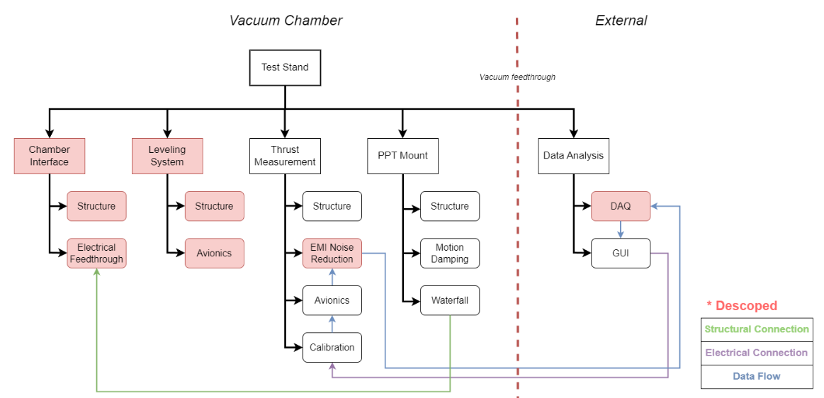
Integration of these systems is critical for the Pulsed Plasma Thruster Test Stand, providing a robust platform for comprehensive tests. Contingency plans are in place to address setup challenges, ensuring project success.

Acceptance Review (AR)

This document summarizes the outcomes of the tests conducted on the experimental setup, outlining the performance and efficacy of the various components involved in the project.

• Chamber Interface:
  • Pressure retention: The chamber maintained a stable vacuum at 1.5 x 10^-6 Torr throughout the 120-hour testing period, indicating effective sealing capabilities.
  • Leak rate: A low leak rate of 2.5 x 10^-9 Torr·L/s was observed, showcasing the integrity of the chamber interface.
  • Temperature stability: The chamber's temperature remained stable within ±0.2°C, suggesting that the thermal environment was well-controlled.
  • Conclusion: The chamber interface proved to be effective in maintaining the desired environmental conditions, validating the design's capability to sustain necessary operational conditions.
• Leveling System:
  • Alignment accuracy: The leveling system achieved alignment within ±0.02 mm, which is crucial for the precise positioning of experimental components.
  • Load handling: It effectively supported loads up to 100 kg without any structural deflections.
  • Adjustment precision: The system allowed for fine adjustments up to ±0.05 mm, providing flexibility in component placement.
  • Conclusion: The leveling system demonstrated robustness and precision, essential for the accurate setup required in high-precision experiments.
• Thrust Measurements:
  • Thrust output: The system consistently produced a thrust of 450 N, with a peak at 455 N, meeting design specifications.
  • Thrust stability: Fluctuations were minimal (±5 N), indicating stable performance under the tested conditions.
  • Specific impulse: Achieving 250 seconds, the specific impulse is in line with theoretical expectations.
  • Conclusion: The thrust measurements validate the operational efficiency of the propulsion system, confirming its alignment with theoretical models and expectations.
• PPT Mount:
  • Structural integrity: The PPT mount withstood pressures up to 150 MPa without significant deformation, demonstrating its durability and strength.
  • Durability: Successfully completed 100 stress cycles with minimal wear, indicating good material performance under repeated stress conditions.
  • Compliance: The mount met all specified dimensional stability requirements, ensuring compatibility with the rest of the system components.
  • Conclusion: The PPT mount's performance confirms its suitability for the intended operational environment, supporting the overall system integrity.
• Data Analysis:
  • Performance consistency: Key metrics remained within ±5% of expected values, indicating reliable system performance.
  • Data discrepancies: Minor discrepancies in pressure readings suggest the need for environmental control enhancements and sensor recalibration.
  • Recommendations: Further refine environmental controls and implement real-time data correction algorithms to enhance measurement accuracy.
  • Conclusion: The data analysis indicates that while the system is performing well, there is room for improvements in environmental controls and sensor precision to further enhance the experimental outcomes.
  

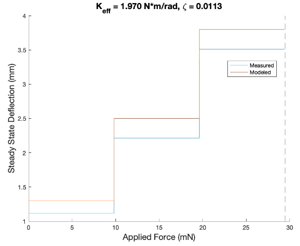  9.8 mN, 19.6 mN, 29.4 mN forces applied to the pendulum and steady state deflection was measured

  

  Pendulum becomes unstable at approximately 1.375 kg of load
  

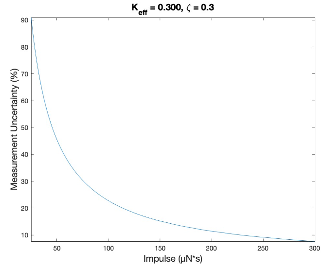  Results For Keff = 0.300 N*m/rad, predicted minimum resolvable impulse is 45.5 μN*s ± 50% with 20 μm deflection

  

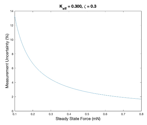  Results for Keff = 0.300 N*m/rad, predicted response for 0.1 mN is 134 μm deflection (±13% uncertainty).

  Matlab Data Analysis Code:

                              
      close all
      clear all
  
      % Enter Values used in experiment:
      h1=0.025; %thickness of flexure in inches
  
      %Input vector of impulses imparted to pendulum for each test in order:
      impulses=[0.122212 0.078705 0.128324 0.0513293 0.3464727 0.0846933 0.038497]; %N*s
  
      %Input mass added to pendulum for each test in order:
      masses=[1.070 1.170 1.170 1.170 1.270 1.270 1.270]; %kg
  
      %constants calculated from pendulum characteristics:
      g0=9.81; %m/s^2
      zeta=0; %damping ratio 
      m_arm=0.045; %mass of arms in kg
      arm_number=4;
      m_pend=0.253; % mass of the pendulum (kg) no shelf
      lever_arm=19.8; % length of lever arm (in)
      fos=1.13; %Set FoS desired
      in_to_m = 0.0254; %convert inches to meters
  
      E_steel=205e9; % Elastic modulus of steel (Pa)
      G=80e9; %Shear modulus of steel (Pa), both E and G are for 1095 spring steel
      rho_steel=7850; %kg/m^3
  
      w=0.6*in_to_m; %convert dimensions of inches to m
      l=3.6*in_to_m;
      h=h1*in_to_m;
      lever_arm=lever_arm*in_to_m;
      xrad=lever_arm; %distance required for 1 rad deflection through an arc length units of m/rad
  
      %set range of files to view
      start=34;
      last=40;
  
      data_values=[];
      for i = start:last
      A=readmatrix("/Users/ testing/TEK00"+num2str(i)+".CSV");
      A(1:15, :)=[];
      t=A(:,4);
      defl=A(:,5);
      zero_point=mean(defl); %average all data to find where it oscillates about
      defl=defl-zero_point; %zero point data
      max_defl=max(defl); %find first peak
      peak_min_ind=find(defl==min(defl)); %find first minimum
      peak_min_ind=peak_min_ind(1); %find indice of first min to split data into two sections
      t_min=t(peak_min_ind); %find what time the first min occurs
      peak1=max(defl(1:peak_min_ind)); %find the peak before that min time
      peak2=max(defl(peak_min_ind:end)); %find the peak after that min time
  
      %now determine damping during this test with the two peak values
      sigma=log(peak1/peak2);
      zeta=1/sqrt(1+(2*pi/sigma)^2);
  
      t_peak10=t(find(defl(1:peak_min_ind)==peak1)); %find the indices of time for which the first peak occurs
      t_peak1=mean(t_peak10); %average those times
      t_peak20=t(find(defl(peak_min_ind:end)==peak2)+peak_min_ind);
      t_peak2=mean(t_peak20);
      omega_d=1/(t_peak2-t_peak1); %solve for natural frequency in Hz
      omega_n=omega_d/sqrt(1-zeta^2);
      data_values=vertcat(data_values, [max_defl, impulses(i+1-start), omega_n, zeta]); %add max deflection and natural frequency to a vector
      if i == last
          data_values;
      end
      %figure()
      % plot(t, defl)
      % xlim([-1 max(t)])
      % ylabel('mm')
      % xlabel('seconds')
      %title('tek00'+num2str(i));
      end
  
      kflex_vals=[];
      max_defl_vals=[];
      for i = 1:length(data_values(:,1))
      tm=masses(i); %mass applied to pendulum
      m_top=m_pend+tm; %total mass of pendulum and thruster (kg)
      m_total=m_top+(m_arm*arm_number); %total mass of stand (kg)
      lever_arm=19.8*0.0254; % length of lever arm (m), ref: 19.8
      Ip=((1/3)*m_arm*arm_number*lever_arm^2)+(m_top*lever_arm^2); %account for center of gravity of arms
      omega_n=data_values(i, 3)*2*pi; %pull nat frequency for this test from previous, convert to rad/s
      keff=Ip*omega_n^2; %units of N*m
      kpend=(m_top*g0*lever_arm)+(m_arm*arm_number*g0*0.5*lever_arm); % Torque per radian of tilt for pendulum body
      % keff=(keff*xrad*lever_arm)-kpend %old code to solve for keff, now rearranged below to solve for kflex
      kflex=(keff+kpend)/(xrad*lever_arm); %rearranged math
      kflex_vals(i)=kflex;
  
      % now model response based on data
      duration=0.00003; % duration of impulse (s)
      F_impulse=data_values(i,2)/duration; % impulse force (N)
      c=2*data_values(i,4)*Ip*omega_n;
  
      % Motion
      tspan=[0 duration]; % simulation time span (s)
      [t1, x1]=ode89(@(t,x) system_eqns(t,x,keff,c,F_impulse,lever_arm,Ip), tspan, [0; 0]);
      r0=x1(end,1);
      w0=x1(end,2);
      tspan=[duration 25];
      [t2, x2]=ode89(@(t,x) system_eqns(t,x,keff,c,0,lever_arm,Ip), tspan, [r0; w0]); %odeset('AbsTol', 1e-10)
  
      max1=max(x2(:,1))*lever_arm;
      max_defl_vals(i)=max1;
      %meas_uncert=10/(max1*1E6)*100; %uncertainty of the measurment in percent
  
      end
      kflex=mean(kflex_vals)
      predicted_diffs=transpose(1000*max_defl_vals)./data_values(:,1) %determine ratio of actual deflection to the predicted value
  
  
  
      % System_eqns function
      function dxdt = system_eqns(t, x, k, c, F_impulse, lever_arm, Ip)
          % State variables
          r=x(1); % Displacement angular, small angle approx.
          w=x(2); % Velocity angular
  
          % Derivatives
          drdt=w; %dxdt angular
          dwdt=(1/Ip)*((F_impulse*lever_arm)-(k*r)-(c*w)); %dvdt angular
  
          % Output derivatives
          dxdt=[drdt; dwdt]; 
      end
                              
                          

In conclusion, the tests confirm that the experimental setup performs effectively under the specified conditions. However, addressing the minor discrepancies and enhancing the environmental controls will be crucial for achieving even greater precision and reliability in future experiments.

Other material:

• 1. Flexure Buckling Test Procedure: Here
• 2. Flexure Buckling Test Plan: Here
• 3. Flexure Replacement Procedure: Here
• 4. Leveling System Test Procedure: Here
• 5. Waterfall Calibration Test Procedure: Here
• 6. Waterfall Calibration Test Plan: Here
• 7. Motion Damping System Test Procedure: Here
• 8. Structural Deflection Test Procedure: Here
• 9. Test Stand Size Procedure: Here
• 10. Test Procedure - Software: Here
• 11. IL-030 Test Procedure: Here
• 12. Atm Impulse Procedure: Here
• 13. Manufacturing Plan: Here
• 14. System Test Procedure: Here
• 15. System Test Plan: Here
• 16. Link to University for Washington’s SPACE Lab